For around two decades the Risc OS program, “!Composition” was essentially unobtainable. Happily, in April 2024 copies of the old source files, etc., were rediscovered and a fresh version became available again in a ‘revived’ form. Fortunately, this works on modern RO machines and versions of the OS as well as when using old machines or RPCemu. Copies can now be downloaded from the “!Store” repository. For the sake of drawing the attention of newcomers to !Compo, and to celebrate its revival I decided to write some new “Compo Clues” web pages to illustrate the extraordinary range of capability this offers, and how you can employ ‘CompoScript’ to expand the tasks it can perform. This page is the initial new example...

I have also included a link to the source material I created to use in this process, so any Compo user who wishes can see how Compo can be programmed to get the resulting graphics.

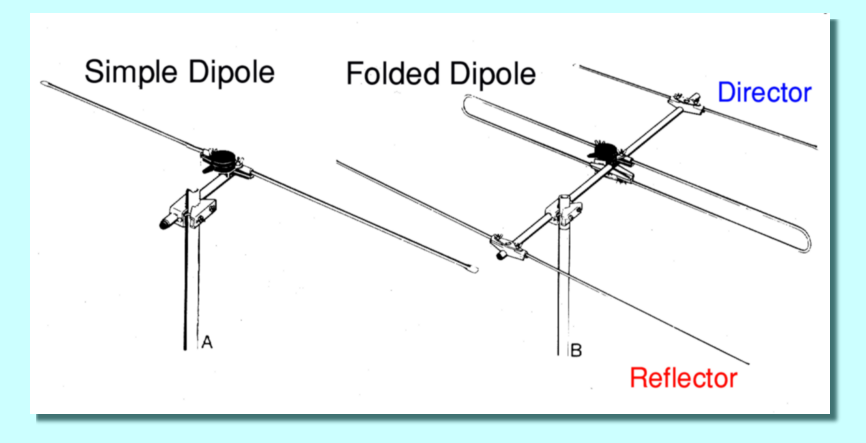
At the time of the new release I was working on trying to analyse and explain the way simple antenna ‘arrays’ work. Rather than get buried with ‘hard sums’ maths I wanted to be able to produce some colourful diagrams that illustrate this, using the example of the simple types of outdoor VHF/FM Radio antennas that are chosen for this purpose in the UK. The drawing at the top of this page shows two examples. One is the simple ‘dipole’ which consists of a single rod of metal, half a wavelength long. The other type adds a ‘reflector’ and a ‘director’. (These terms essentially describe the functions the added elements provide. The ‘reflector’ acts a bit like a mirror - reflecting back towards the dipole. The ‘director’ acts more like a lens, helping the dipole collect from or to ‘beam’ radio signals in a specific direction. These antennas are optimised to operate at frequencies whose wavelength is about twice the length of the dipole.

One remarkable feature of CompoScript is that it not only can essentially automate a set of Compo processes. It can also call in the use of external programs that can also then create or modify or analyse graphical objects on Compo’s ‘canvas’. To illustrate this consider the example result shown below:

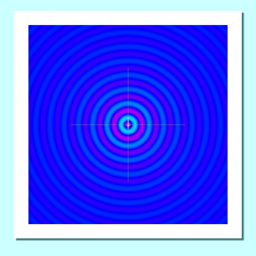
This shows a ‘snapshot’ of an EM sinewave being radiated from a simple dipole. The +ve and -ve half cycles of the waveform are shown in different colours. The two white lines cross at the centre of the dipole. The location of the dipole itself is shown as a small circular object where the white line ‘cross-hairs’ actually cross at the centre of the pattern.

The POV is such that we are viewing the dipole ‘end on’. This shows the radial symmetry we would expect, with the wave energy flowing out in all directions.

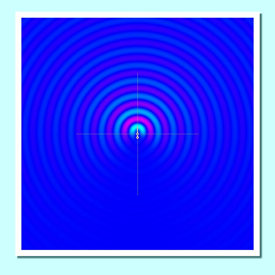
As could anticipate from it’s name, adding a ‘reflector’ element has the effect of bouncing back a lot of the EM energy that would otherwise flow in its general direction. This produces a ‘gain’ in the output if we are in the favoured directions.

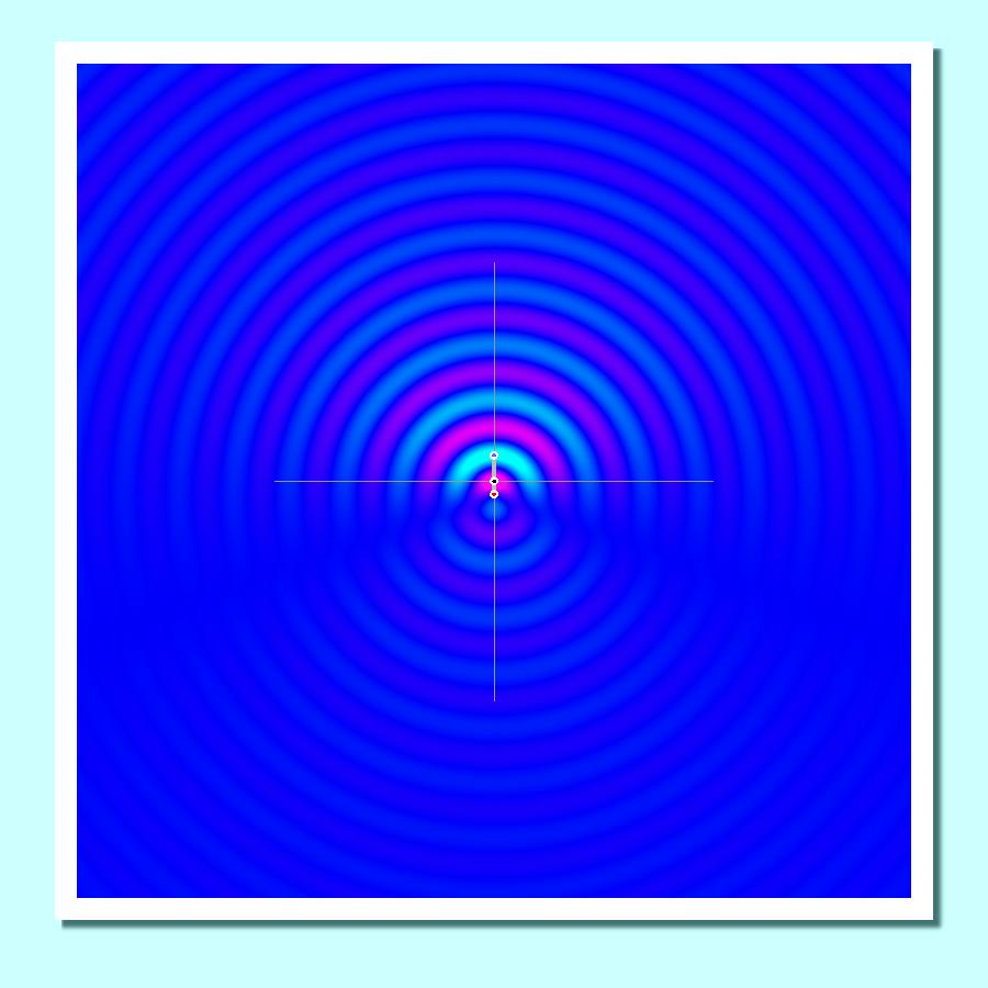
The above plot shows that adding a ‘director’ element enhances this effect of getting ‘gain’ in a preferred direction as the expense of other directions.

Unless you are a radio enthusiast or engineer the precise details of the relevant mathematics don’t matter here. But what is worth noting is that each of the above graphics was generated by Compo and using its ability via CompoScript to ‘call’ other programs. In this case one I wrote in ‘C’ and compiled into runable code that CompoScript could then call to calculate and plot the relevant patterns. The same CompoScript also loaded the small ‘indicators’ at the centre of the plots, put them in the centre, and generated the ‘drop shadow’ effect to make a prettier result on the resulting webpage.

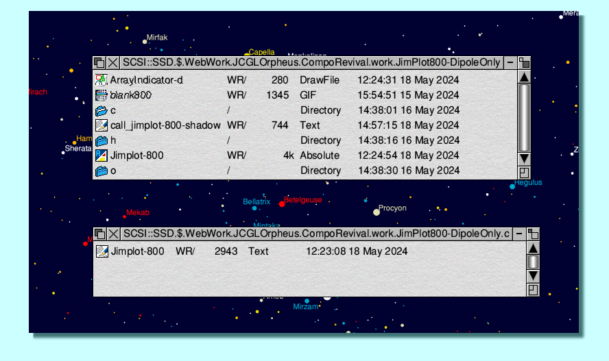
The overall structure of the use of CompoScript and the related files is illustrated in the above screengrab from my ARMX6. To run any of the example processes you open up a !Compo canvas (window) and then drag-and-drop the text file whose name begins with “call_”. The content of that file is the series of CompoScript instructions that then guides the process that follows. Here I’ll use the “Dipole-Only” example, but the others work in the same way.

The initial command is: makecanvas 900 900 13434879

This sets the size of the Canvas to 900 x 900 pixels and the colour to “13434879”. This is the decimal value corresponding to the required hex form as RRGGBB – i.e. hex CCFFFF.

The next section of code loads and selects the blank white gif file “blank800”. The location given for it is a filer location relative to the “call_” file. Having loaded this the move50 50 50 moves the resulting white square to a place on the canvas that is 50 pixels from the bottom left corner of the canvas. It then selects this graphic object as the item to be manipulated.

The next line is: star "WimpTask <.composcript$dir>.Jimplot-800 <.selected.imagebase>"

That calls some code which was complied from an Acorn ‘C’ program. Again the file is in a specific location relative to the “call_” file. The content of this code then does the bulk of the work required to generate the required pattern in the resulting image. The ‘C’ source code is listed in the file “Jimplot-800”. Once this process ends the redraw CompoScript causes the complete field pattern to be shown.

The script continues by adding and positioning a drawfile that then serves as an an indicator of the locations etc., of the antenna whose near-field pattern has been plotted. The commands that follow then adjust the positioning and adding drop shadows to give a prettier result.

Note that the computation process which plots out the field pattern has to calculate and plot hundreds of thousands of pixel values! Hence you may see the hourglass for a few seconds as this is done! (And the more elements in the antenna, the longer this will take!) But the result overall is that Compo can produce an attractive, complex graphic in an automated way that can be driven by a relatively simple program written in some other computer language like ‘C’ or BASIC. You aren’t limited to what the CompoScript itself can calculate. It also provides a doorway to adding your own processes and using Compo as a ‘rendering and control system’. (Yes, Iall being well, ’ll deal with ‘control’ on a later webpage...)

Although I’ve not done so here, this can also be extended. For example, !Compo can create animated images. So it would also be able generate an equivalent to the above where the E-field wave patterns would ‘ripple’ outwards, mimicking how the radiation propagates as time passes! The snag being that this would take longer to create. But because the process would be automated, you could go and have a cup of tea while this was being done! :-)

July 2024