In general I’ve tended to use the old RO Application !Tau to create the familiar kinds of X/Y graphs with a rectangular geometry. It works very well for generating DrawFiles showing the resulting graphs. For some special purposes I also often use my old !DrawGen program which offers more flexibility in what you wish to draw or plot. For example, this can draw ‘Polar’ line graphs which !Tau is unable to create. However my previous article on the Revived version of !Compo featured polar patterns of a kind which neither of these applications can easily generate! These are forms of ‘Colour Field’ graphics where the value of some quantity is displayed as a function of two variables – (x,y) if we wish to produce a rectangular field, or radius/angle if we wish to generate a polar colour field.

The aim of this article is to example in more detail how we can use CompoScript as a means to plot almost any kind of graph we might wish to produce, via using it to feed in data from an external program. To do this I’ll continue to use the behaviour of a simple antenna, but in terms of how to create a standard polar linear plot of antenna patterns which show how the antenna’s gain or sensitivity varies with direction.

    You can get a zip of this program here.

In this case, when the program is run it will look for the input data in a file and then plot what the data defines. I’ve supplied a test file, called DataScaledToPlot for this process, and the program will look for this on your RamDisc. So before you run the program drag-and-drop a copy of this file onto your RamDisc. You can run the actual program by dropping the script file onto the open Compo canvas.

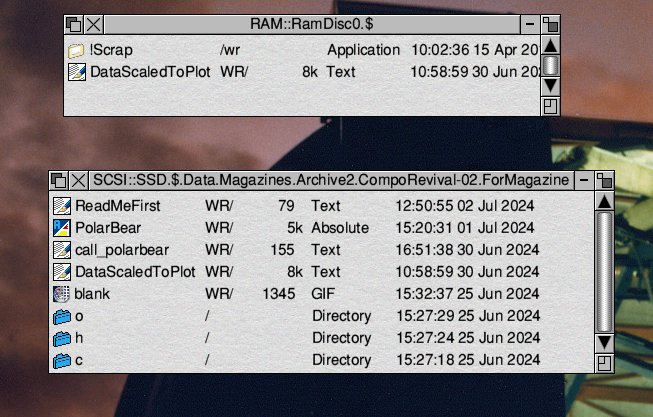
I’ve adopted a policy of giving these script files a name starting with “call_”. This is to help distinguish them in a filer window from other files. In essence using the prefix as a reminder of what type of file they are. The above illustration shows the directory that holds all the relevant files, etc, for this example of using CompoScript. So far as the filer is concerned these files are just text files, so you can use name them however you find convenient. For the present purpose I called the script file “call_polarbear”.

The content of this file is:

    #CompoScript
    loadimage <.composcript$dir>.blank
    moveto 20 20
    star "WimpTask <.composcript$dir>.PolarBear <.selected.imagebase>"
    redraw
    end

This selects the bitmap object “blank” (which is in this case an 800x800 pixel, white GIF file), loads it onto the canvas, and then moves it so that its bottom-left corner is 20 pixels above and to the right of the bottom left corner of the canvas. It then leaves it identified as the target for any Compo process which may then be requested.

Note that the specified locations of files in the above lines are all relative to the location of the directory which contains the CompoScript file that was dropped onto the canvas. This ensures that if we keep the files together in a directory the set of files can be copied or moved elsewhere and still function provided that their relative locations remain unchanged.

The ‘key’ that then opens the door to access the object on the canvas is the line:

    star "WimpTask <.composcript$dir>.PolarBear <.selected.imagebase>"

In this example “PolarBear” is an Absolute code file which I compiled from a program I wrote in AcornSoft ‘C’. (Hence the subdirectories, ‘c’, ‘h’, and ‘o’ in the directory.) The star command executes this code as a simple WimpTask. The “selected.imagebase” enables the PolarBear program to locate and access the memory locations of the sprite on the Compo canvas. (Bitmaps loaded into Compo all get represented in its ‘Sprite layer’ as sprite format data in memory.)

I won’t list all of the ‘c’ code here, I’ll just point out the key aspects of the process. The process starts by using a ‘get_sprite_start()’ procedure to discover where the sprite’s data starts in memory. Then ‘get_sprite_size()’ discovers the width and height of the sprite in pixels. The image data for sprites is held by Compo as a series of binary values which we can treat as a set of 4 bytes per pixel with the ordering: [XX][BB][GG][RR] - i.e. RGB colour values. Given this info, the program can now peek and poke to read and/or write the colours of chosen pixels.

The above outlines how we can use CompoScript to enable an external program we have written to analyse and/or change the image to be held and displayed by that sprite. (And hence also then saved when processed.) How we choose to exploit this is a matter of what we wish to achieve. In effect, the potential is open-ended. The initial use I demonstrated was the ability to create a polar patterned ‘colour field’ showing the relative field levels around some simple radio antennas. However there is one remaining aspect of this that we need to deal with... where are we???...

When drawing graphs we normally start by choosing some axies to represent the related quantities. Most often the choice is a rectangular geometry with (x,y) axies to show how one quantity varies with another. However – as the previous antenna example showed – in some cases a ‘polar’ linear plot gives a more appropriate view. Hence now using CompoScript to create polar linear graphs of antenna patterns of the gain/sensitivity versus angle of arrival (or emission).

The computer memory area the program can now access represents the sprite data as a one-dimensional series of values (unsigned ints) located via a series of address values - i.e. Not a 2-dimensional array, let alone some kind of magic circle! Hence we need a method which lets us convert between the location of a pixel’s colour value in the sprite data held in memory and a place on the visible image. The ‘c’ source code in the PolarBear file provides an example of how this can be done.

Two subroutines: get_sprite_size() and get_sprite_start() return values for height, width, and size (in pixels) of the object’s sprite data area. In terms of (x,y) units of a rectangular graph we can the set a value

    ncenter = width*height/2 + width/2;

which is the address in the sprite data of the image’s central point (pixel). Having obtained this value the subroutine

    int thispixel(int xin,int yin)
    {
      int nout;
      nout = xin - yin*width + ncenter;
      return nout;
    }

In this case I’m writing directly to pixels on the selected object. But if you wish, plotting data points on the graph could be done via using another small bitmap (or DrawFile!) object as the marker for each data point, positioned by a suitable moveto x y for each point being plotted. That offers some ways of being more flexible in terms of choice of markers and get a better appearance. However for now I’ll use the more direct approach.

The first line of the DataScaledToPlot file contains two numbers. The first is number of data sets to read. The second is how many data points there are for each direction (angle). The values are scaled to fit the sprite and its calibration circles. For the example I have provided data lines for 360 angles, each having two points whose radial distances are specified. This lets the plot show the antenna patterns of two different antennas. Note that the angles are in degrees, and that the radial ‘sizes’ for the two patterns are pre-scaled to fit the size of the axies and sprite.

For the sake of demonstration and distinguishing one polar pattern from the other the two sets are then plotted in different colours using ‘markers’ with different shapes.

The above image shows the result this creates on the Compo canvas. If we zoom in the view we can see more clearly the difference in the plots for the two polar patterns of values vs angle.

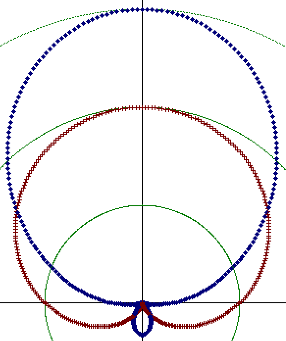
The use of different colours and shapes for the two angle-vs-radial length helps to visually distinguish one pattern from the other.

The main purpose of this article is simply to demonstrate an example of how Compo can be used to render graphs like the polar form given suitable data. I used a program compiled from ‘c’ but other languages could be employed, and then connect to Compo for rendering of the results. Better-looking results can also be employed to get smoother results, etc. I haven’t bothered to try and get a better appearance by various possible means because the aim here is just to serve as a simple example of being able to plot alternative formats of graphic via CompoScript.

In practice the type and visual quality depends on the format that best suits the user and the nature of the data! I hope to consider some other examples in future, and the potential for reversing the process entirely and reading data from graphics!

1500 Words     
2nd Jul 2024